Satellite Image Classifier
Project Source Code: github.com/snmca/satimg-classifier
This project was undertaken as the capstone project of Data Mining (CSC 503/SENG474) at the University of Victoria. It was completed with a group of students. Individual contributions can be found in the provided commit history.
Introduction
The work of prospecting for mineral deposits is complicated and can be dangerous. In some cases it can be harmful to the environment and human health. Current techniques depend on specific geological knowledge, and utilize a combination of magnetic, gravimetric radiometirc, and seismic methods. Our work proceeds from curiosity; can AI assistance be used to learn generalizable patterns — as of yet unknown to human geologists — that emerge in surface features, which may be highly predictive in identifying useful mineral deposits?
This project was conceived, in part, to take advantage of the extensive Landsat dataset, which is freely available and contains over 8 million Earth observation scenes taken over the past 50 years.[1]
Landsat images are very high resolution, as such, Convolutional Neural Networks were chosen as the primary learning agent for this project. Convolutional Neural Networks have proven to be very effective in image classification tasks.[2] Of particular interest to this project is the ability of CNNs to quickly reduce the resolution of an image, while preserving learned patterns. This is useful for our project, as the Landsat images are very high resolution, and would be difficult to train on using a consumer GPU. The Landsat dataset was combined with a dataset of known mineral deposits to generate training labels for supervised learning; the label of each image indicated the presence or richness of minerals in the image.
We aim to train Convolutional Neural Networks to achieve 80% validation accuracy on the binary classification problem, and a Mean Absolute Error of ≤ 0.1 on the regression problem.
Problem Formulation
The problem formulation step encompasses the bulk of the work. This step prepares the data for the model to train on. The particular ways in which the dataset is chosen, labelled, and prepared effect what the model will learn. These decisions are made with the goal of constraining the problem in such a way that the model will learn to solve the problem as formualted in our minds. Each formulation rests on a particular philosophy of what should be learned, and each has its own strengths and weaknesses.
We formulated the problem in two ways: binary classification (2.2), and regression (2.3). Both approaches shared much of the same acquisition and preprosccesing pipeline as described below.
Data Acquisition & Preprocessing
We acquired the entire set of approximately 45000 band 7 images from Landsat 4 of the public Landsat dataset on Google Cloud Platform. We chose band 7 (2.09-2.35μm) because it uses a Thematic Mapper sensor to capture light in frequencies optimal for identifying hydrothermally- altered rocks associated with mineral deposits.[3] These images are each approximately 7500x7500 pixels in a single colour channel, and are taken at regular locations on a 2x2◦ latitude-longitude grid.
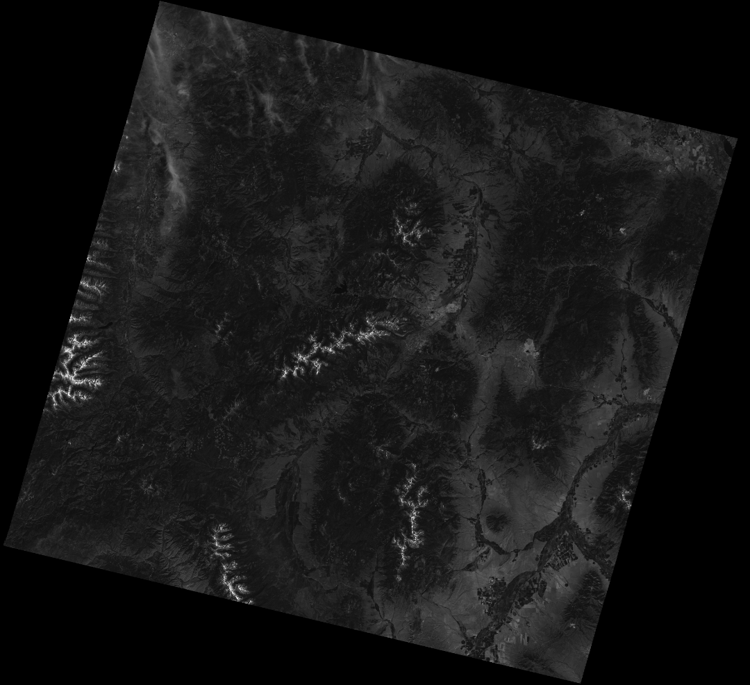 Figure 1: An example Landsat image in band 7
We also acquired a dataset of approximately 350000 mineral deposits, each including the deposit’s coordinates and the types of minerals present.
We automated the image downloads using a bash script. This script used the bash utility ImageMagick to down-sample each image from 7500x7500 to approximately 512x512, to allow for training on consumer hardware. The corresponding metadata file for each downloaded image was also obtained, containing information such as the coordinates of the image corners. The download took approximately 6 seconds per image, for a total download time of approximately 75 hours.
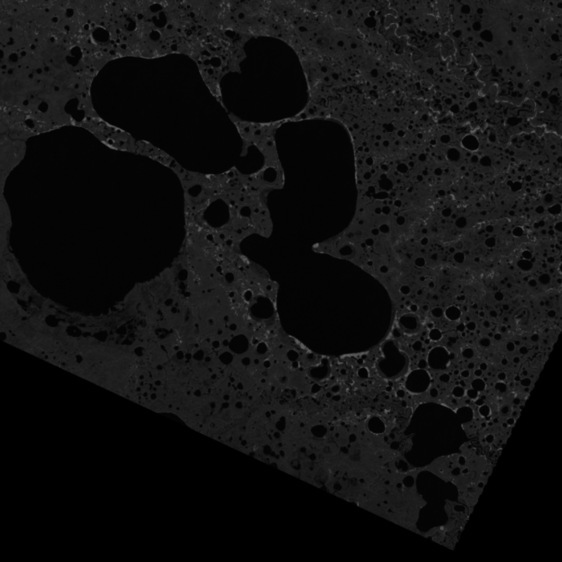
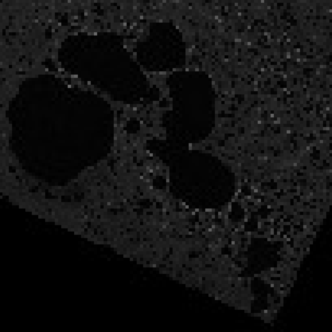
Several different algorithms from were experimented with: resizing, rescaling, and sampling. Resizing and rescaling use similar iterative processes of averaging neighboring pixels to effectively compress the image while reducing quality. Sampling is a more direct approach which simply selects a subset of the pixels evenly from across the input image. This is the lossiest of the three methods, but is also the fastest. The results of these three methods are shown in Figure 2.


Labels were created for each image using an algorithm accelerated by a k-d tree of mineral deposit locations; the k-d tree was used since k-d trees provide significant speedup for queries on spatial data.[4]
Efficient label creation was nontrivial since it required identifying which mineral deposits were present in each image, and the images were neither axis-aligned nor perfectly rectangular. To address this, the label-creation algorithm first computed the enclosing circle of each image, then queried the k-d tree for the set of deposits present in the circle; brute force was then used to test which of these deposits were within the convex polygon of the image. This method provided a speedup of 20x over the naive approach.
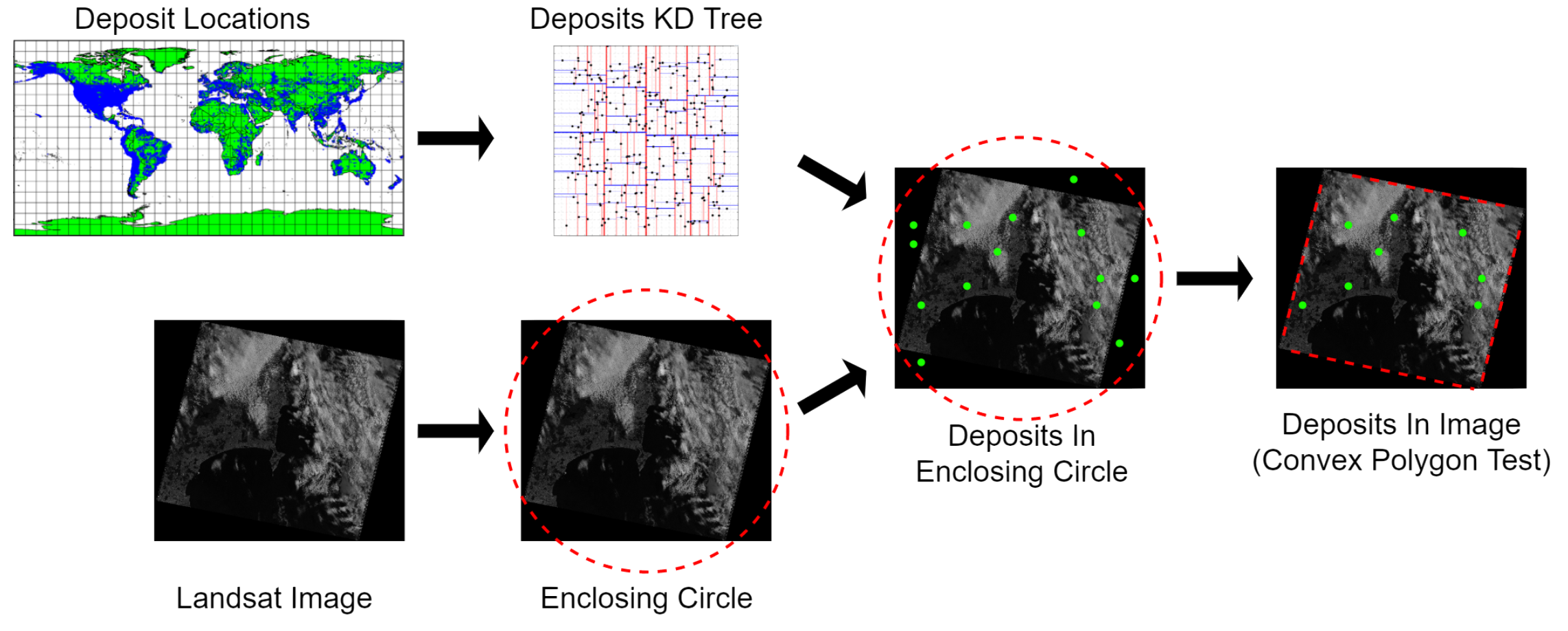 Figure 3: Label creation pipeline
Having obtained the set of deposits present in an image, separate labels were created for binary classification and regression. The binary classification labels indicated whether any minerals were present in the image, and the regression labels indicated the mineral richness of the image. The richness score was computed as the log transform of the absolute count of deposits in the image, normalized to the range [0,1]. The log transfrom was used to reduce the skew of the regression values.
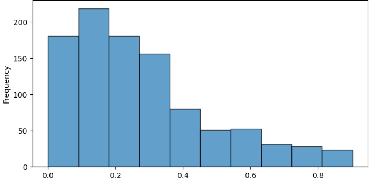 Figure 4: Distribution of log-normalised richness scores
Location Buckets: Since Landsat images are taken at regular intervals, and our dataset contained several images at each location, it was necessary to ensure that no location appeared in both the training and testing sets simultaneously. To achieve this, the images were grouped by location, resulting in approximately 6000 unique location buckets.
Cloud Cover: Having grouped the images by location, the images in each bucket were sorted by average pixel brightness, which for band 7 images effectively sorts by degree of cloud cover. This permits the selection of training images having less cloud cover.
Ocean Masking: Images in location buckets over the ocean were then removed, to ensure that our models did not learn to simply detect land. The Python library Geopandas was used to load a geospatial dataset containing the polygons of the boundaries of all land on Earth; this dataset was then queried to determine whether each image’s centerpoint was over land.
Training + Testing Sets: To prevent our models from simply learning the underlying distribution of training labels, we ensured that the ratio of class labels in the training set was balanced. In binary classficiation this is trivial, we enforce that the training set be comprised of 50% positive and 50% negative labels. In the regression case, the set of all examples has some underlying distribution shown in figure 4. The training set is then sampled randomly (without replacement) from this distribution, and therefore comes to have a very similar distribution. The remaining images are used as the validation set. This ensures that both sets have a near-identical distribution of labels.
The training and testing sets were drawn from the set of all images such that at least one image from each location bucket was included. The training set was then randomly sampled from this set, and the remaining images were used as the testing set. All experiments used a 80/20 split between training and testing sets.
Padding: Finally, since the Landsat images vary slightly in size and are not perfectly square, each image was padded to 512x512 pixels with black pixels, and all pixel brightnesses were normalized to the range [0,1].
Binary Classification
The binary classification problem setup was the first to be designed. It represents the simplest formulation of the problem, and our naive initial understanding. The primary goal of this problem was to determine whether a model trained on the dataset described above could learn anything relevant to the problem which would enable it to perform better than chance. To this end, examples with binary labels were prepared for the model as described above.
This approach initially proceded from the assumption that mineral deposits would be sparsely located throughout the world, and that their presence might correspond to certain easily detectable surface features. However, when the labelled location buckets were later plotted on a world map it became obvious that there was a clear preponderance of positive labels over land. Given the large surface area covered by each image almost all images contained at least some small number of desposits.
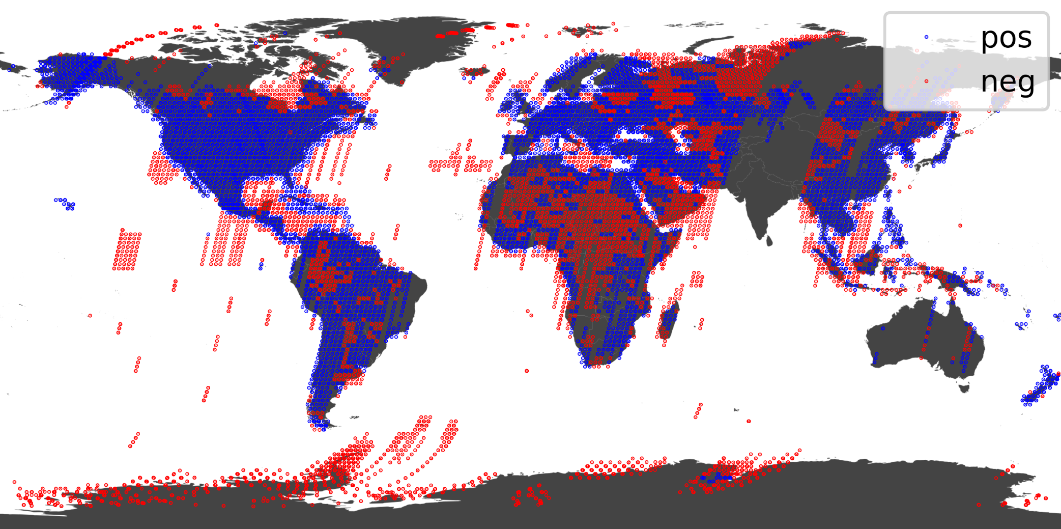 Figure 5: All labelled location buckets
Additionally, negatively labelled images do not necessarily mean that there are no mineral deposits in the region. In fact, this is a major philisophical problem with the problem setup. Many of the false positives that the model will produce may in fact be true positives representing new deposits which the model has successfully identified. Without any way of independently verifying the presence of these deposits we are unable to truly evaluate the model’s performance, and the model could never further learn from these examples. Nevertheless, this problem formulation does allow us to successfully determine whether our dataset contains information which is learnable by a CNN.
Regression
The regression problem was designed to address the issues with the binary classification problem, and sought to investigate the feasibility of the practical application of our methods. In practice, a predicted richness score is more useful than a binary prediction when choosing a location to dig for minerals. The regression formulation also addresses the problem of whether negative examples are really negative: if a regression model achieves a low error when trained only on examples containing known deposits, then predicts a high richness score on an example containing no known deposits, it may indicate the presence of undiscovered deposits.
Background and Related Work
Much of the previous work done to integrate satellite and aerial photography into the mining industry has had the goal of better assessing geographic factors relevant as obstacles to construction and extraction.[5] As well as to predict the likely extent of damage to the natural landscape, for instance, to determine if much tree cover would have to be removed. Other work at automatically detecting minerals from orbit has been limited by the sensor capabilities of satellites, indeed typically only those sensors with very high resolution and particular imaging wavelengths are useful for geological applications.[6]
Other work has incorporated AI in the development of maps, and to search for particular features and reflectances which are already known to geologists to correlate with particular kinds of deposits.[7]
Our work proceeds from the question; can new patterns useful in predicting the location of deposits, as of yet unknown to geologists, be learned by ML agents? Our work is limited by the resolution of the data and our computing power. A more exhaustive search of this question would train on multiple EM bands, and the full resolution available; and would likely achieve more impressive results.
Methods
This section describes the experimental methods used to train the CNNs, and tune the CNN archi- tecture and hyperparameters. To reduce the size of the search space of possible architectures and hyperparameters, a heuristic was applied: first a set of candidate architectures were trained and evaluated; then only the architecture exhibiting the best performance was subjected to hyperparameter tuning.
Model Architecture
Convolutional Neural Networks are a type of deep neural network which are well suited to image classifications tasks. They are composed of a series of convolutional layers designed to quickly extract ever-higher level patterns from the data. The convolutional layers are followed by a series of dense lay ers which perform the classification task. The final layer is a single ouput neuron which produces a value in the range [0,1]. In the binary classification case this is taken to be the predicted probability that an image contains at least one mineral deposit. In the regression case this is taken as a prediction of the extent of mineral richness.
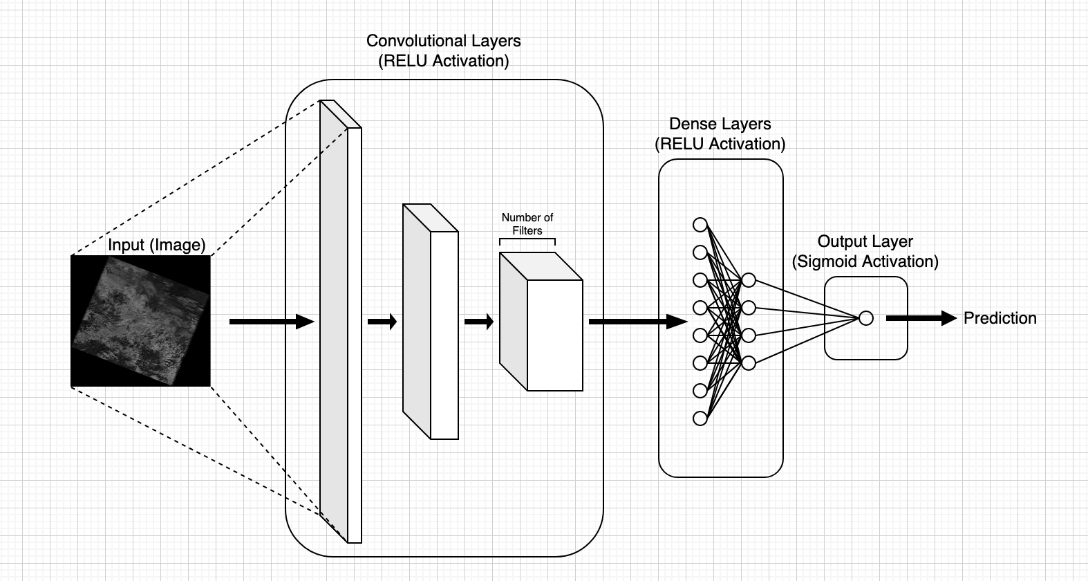 Figure 6: Generic CNN architecture
Convolutional layers each have assosciated filter(s). Each filter is an f x f grid of weights, and an assoscitad bias. A convolution operation involves "sliding" the filter over the layer’s input (for the first convolution layer the input is the example image itself). The amount by which the filter is slid at each step is determined by the stride. For each location of the filter against the input layer, an element-wise multiplication is performed and summed to produce a single output fed into the following layer. Equation 2 describes the 2D convolutional operation in the case that the stride is 1 in each dimension. Where Z is the convolutional output, W is the matrix of filter weights, X is the input layer, and b is the bias.
Several nonlinear activation functions are available to be applied to the output of each layer. The most common, and most successful in this project was the Rectified Linear Unit (ReLU) function. The ReLU function is defined below in equation 3.
It is common to also include a pooling layer after each convolution. Pooling is a technique which can reduce the resolution of the output from the previous layer, without introducing any further trainable parameters. This simplifies further training while preserving the most important features of the input. Commonly, max pooling layers are used, their behaviour is described in equation 4.
To prevent overfitting, L1 and L2 regularization can be applied to the weights of each layer. These regularizations are penalties added to the models loss function to discourage large weights. This prevents the model from depending on any particular features too much. L1 regularization is less aggressive, it is described in Equation 5. L2 regularization is more aggressive and is described in Equation 6. In both cases λ is a hyperparameter which controls the strength of the regularization.
We additionally found that batch normalization was useful in increasing model performance and possibly improved training times. Batch normalization is a technique which normalizes the output of each layer to have a mean of 0 and a standard deviation of 1. This has the effect of preventing any particular layer from dominating the training process. Batch Normalization is described in Equation 7, where ε is a small constant to prevent division by zero.
Dropout layers were also added to the model architecture between the convolutional and dense network components. Dropout layers are intended to prevent overfitting by randomly selecting a fraction of a layers neurons to ignore during a training iteration. This has the effect of forcing the model to learn to perform the task without relying on any particular neurons. The fraction of neurons to ignore is controlled by the dropout rate hyperparameter, p. Each neuron has an even chance to be dropped. This is described in equation 8.
In summary, a convolutional neural network consists of a series of convolutional layers, followed by a series of densely connected layers. Each convolutional layer may consist of many independent feature maps, each with its own filter. The output of each convolutional layer is the a matrix with resolution diminished by the stride and size of the filter according to equation 9, in the 2D case. Where d is the input dimension, f is the filter size, s is the stride, and p is the padding (typically p = 1 in our experiments).
The output of the convolutional layers is then flattened into a vector, and fed into the dense layers. The forward pass step of the convolutional layers can then be described by equation 10. Where K is the number of feature maps in the previous layer, shown here in a 2D n × n example. And the forward pass of the densely connected layers is familiar, shown in equation 11.
The result of the final dense layer is transformed by the sigmoid activation function, in order that all network outputs be in the range [0, 1]. The sigmoid function was found to be the most effective activation function for our task and is described in equation 12.
The candidate architectures each had a unique combination of two architectural characteristics: the complexity of the convolutional network, and the complexity of the dense network. "Big", "medium", and "small" configurations were defined for the convolutional and dense networks, and every possible combination was trained to convergence, for a total of 9 candidate architectures. Since the convolutional network extracts abstract features of the image, and the dense network performs classification using those features, varying these architectural characteristics independently allowed us to investigate the nature of the patterns relevant to the problem. For example, if a deep convolutional network provided no improvement over a shallow one, it could indicate that the general, high-level features of Landsat images carry little information relevant to the problem of mineral richness.
Hyperparameter Tuning
The hyperparameters described in the previous section were varied over ranges which were determined to be sensible for each, as determined by some brief preliminary experimentation. The hyperparameters were then tuned using a search over the ranges. Optimal values were determined by training each model for 200 epochs, and selecting the hyperparameter values which produced the lowest validation loss.
Model Evaluation
The binary classification problem trained the model using the binary cross entropy (or log loss) loss function, shown in equation 13. The regression problem trained the model using the mean absolute error (MAE) loss function, shown in equation 14.Where y is the true label, and o is the model output. Both models were trained using the Adam optimizer, which is a variant of stochastic gradient descent. The Adam optimizer is a popular choice for training deep neural networks.[8] In practice, each loss function may be modified by the regularizations described in the previous section.
Prior to the architecture and hyperparameter tuning, performance baselines were obtained for the binary classification and regression models; this was an important preliminary step for evaluating later model performance, since it allowed us to measure the improvements provided by each optimization.
These baselines were obtained by training the medium-medium CNN configuration on examples having randomized labels for the training set, to ensure that the training set contained no learnable information relevant to the problem. The binary classification baseline was 50% validation accuracy, and the regression baseline was a MAE of 0.127.
Results
This section presents the results of the architecture tuning, hyperparameter tuning, and other experiments performed for the binary classification and regression problems.
Binary Classification
After the baselines were achieved and prior to architecture tuning, a simple, naive CNN was trained for binary classification using the correct, non-randomized training labels; this model achieved a validation accuracy of 65%. The architecture and hyperparameter tuning improved this value by close to 10%. Of the candidate architectures, the large-large configuration performed the worst and the medium-small configuration performed the best. In general, shallow, wide networks tended to perform better for the binary classification problem. The maximum accuracies achieved by each candidate architecture before hyperparameter tuning can be found in table 1.
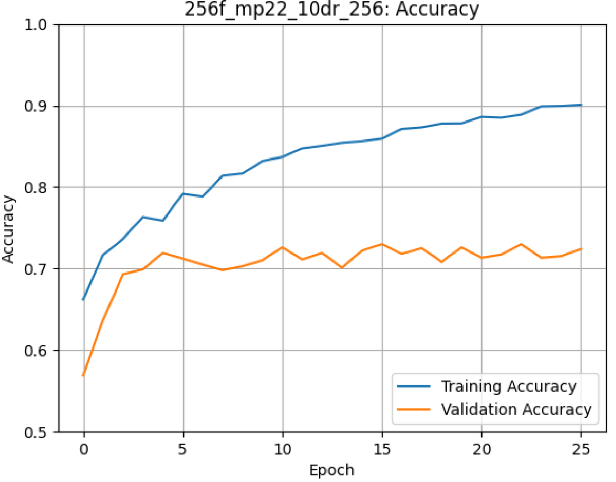
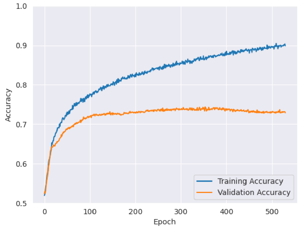
Table 1: Candidate Architecture Accuracy Results, Binary Classification
| Architecture (Conv-Dense) | Accuracy |
|---|---|
| Small-Small | 0.721 |
| Small-Medium | 0.683 |
| Small-Large | 0.712 |
| Medium-Small | 0.732 |
| Medium-Medium | 0.691 |
| Medium-Large | 0.698 |
| Large-Small | 0.724 |
| None-Medium | 0.718 |
| Large-Large | 0.676 |
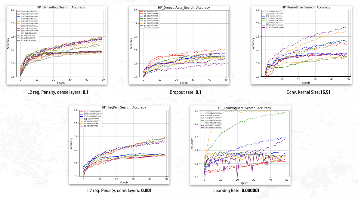 Figure 8: Hyperparameter Search
Hyperparameter tuning provided only trivial accuracy benefits of less than one percent.
Regression
The best model obtained for the binary classification (Medium-Small) problem was reconfigured for the regression problem and trained to convergence. This model exhibited an improvement over baseline of 8.2%, with a baseline MAE of 0.127 and a trained MAE of 0.117. The training curve is shown in Figure 9.
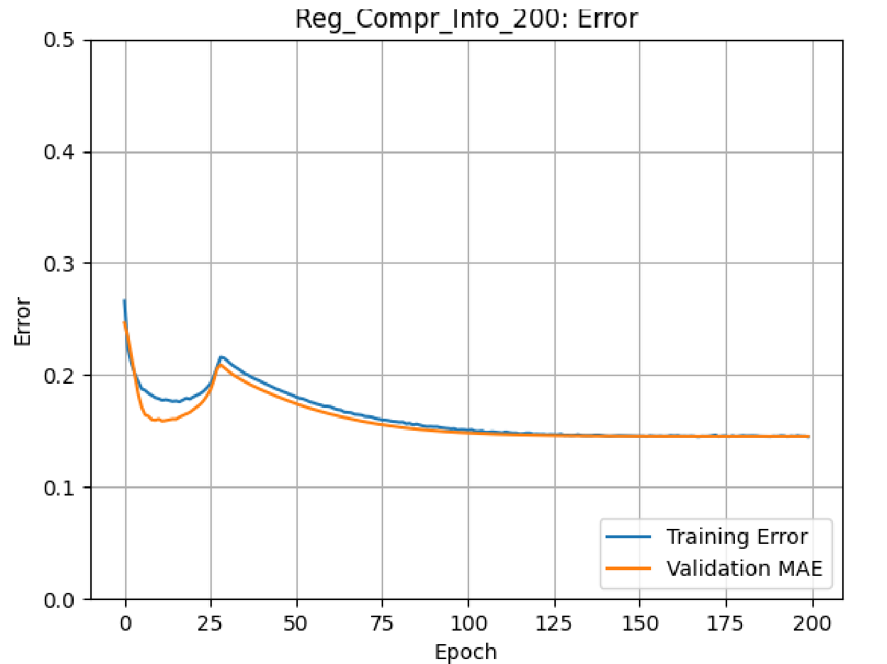 Figure 9: Medium-Small Model Training Curve on Regression Problem
Discussion
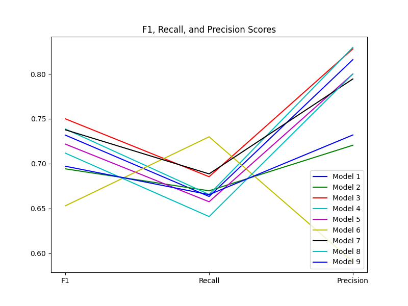
The best F1 score produced for binary classification was 75%, achieved using the medium-small model, with a recall of 69% and precision of 82%. These results suggest that the model is accurate in identifying positive cases with high precision while keeping false positives relatively low. Figure 10 shows the observed F1, precision, and recall scores for all models. These results also show that the medium-small model performed the best, and that the large-large model performed the worst.
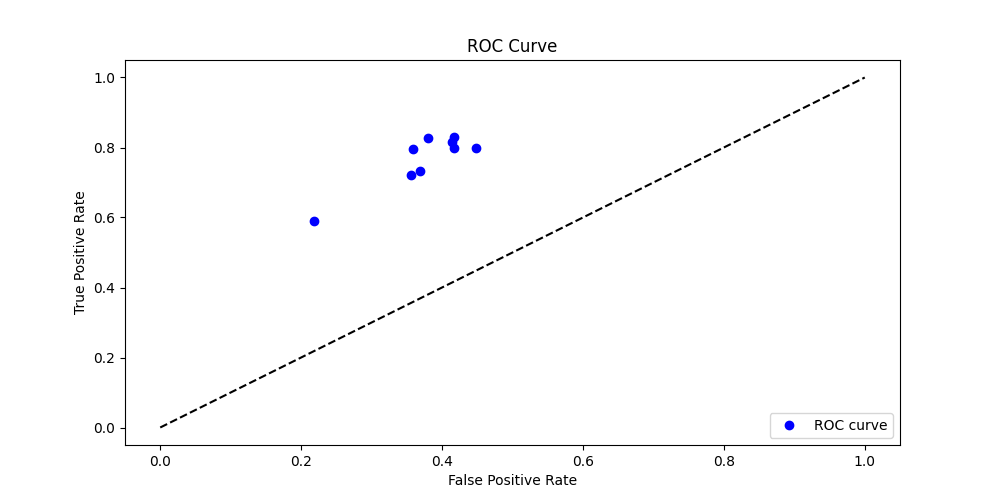
A Receiver Operating Characteristic (ROC) plot was created for more information about the model’s performance. It was only plotted for the binary classifiers at a single threshold. The ROC plot was created by plotting the true positive rate (TPR) against the false positive rate (FPR). This shows that the models were indeed good classifiers, and had a high true positive rate of around 0.8 with a lower false positive rate of around 0.4.
Interestingly, deeper models had longer training times without a significant improvement in validation accuracy, and regression training showed a double-descent pattern. The highest validation accuracy observed in the experiments was approximately 73%, with further hyperparameter changes not leading to significant improvements. This may indicate that the model was learning almost all available information exposed to it in the dataset, and that the use of higher-resolution images could expose more information to the model and improve its performance.
Since we cannot be sure that our negative examples are in fact free of mineral deposits, but only that they are free of known mineral deposits, we note that our false positives are suspect. It is possible that the false positives in fact indicate the presence of undiscovered deposits.
Although we failed to achieve our goals of 80% accuracy for binary classification and 0.1 MAE for regression, we did observe significant improvements over baseline in both cases. And since we removed many sources of error during preprocessing, we believe these improvements demonstrate that our models were able to learn patterns indicative of the presence or richness of minerals in the images.
Limitations
These results are limited by the ambiguous quality of the mineral deposit dataset, which is incomplete. And although we manually verified the locations of a random sampling of the deposits, we did not exhaustively verify the dataset. Any errors in the minerals dataset would be expressed as inaccuracte labels in our dataset, and would reduce the reliability of our models. And since some of the mineral deposits are located at open mines visible from space, our model may be learning to simply detect mines, to some degree. Our results are also limited by the consumer hardware on which we trained our models; although we saw little performance benefit from larger models, much larger models and more powerful hardware may still obtain better performance even on our downsampled dataset.
Future Work
A further improvement would be to replace downsampling with partitioning of source images, breaking them into many examples preserving the original pixels, and computing new bounding boxes and labels for each. However, automating this partitioning may be nontrivial since each Landsat image is superimposed on a black enclosing square, at inconsistent rotations relative to the square. Indeed, if a technique was developed to automatically remove the black bounding box of each image, we might see a performance improvement from this alone.
Since we were able to demonstrate significant learning in the naive binary classificatiaon case, we could focus more on the regression problem, since we believe the regression problem has greater potential for practical applications. In particular, we would attempt to achieve low error on the set of images each containing at least one known mineral deposit, then use the trained model to predict the mineral richness of images having no known deposits, in order to "prospect" for undiscovered deposits.
Since we were constrained by the amount of computing power we could apply to the problem, we could purchase more compute, or try alternate problem formulations. Training times were too long to attempt many approaches, and downsampling was required to avoid memory exhaustion; however, progress could be made by exploring ensemble or boosting techniques and having access to more GPUs and better hardware.
Another promising direction may be to create alternate labels indicating the presence or richness of particular mineral types in each image, since the mineral deposits dataset specifies the mineral types present at each deposit. Such experiments could investigate whether our methods are better suited to the detection of particular mineral types. We might also manually inspect our dataset and remove examples containing open mines visible from space, to ensure that our models are not learning to simply detect mines; note however that this would require a significant time investment.
Finally, obtaining higher-quality labeling data would be the next step for this project. There are some ambiguities in the minerals dataset, and it’s unclear how exhaustive it is. Therefore, obtaining more comprehensive labeling data would improve the accuracy of the models. For example, we might seek out other datasets similar to the mineral deposits dataset, and combine them.
Conclusion
Experiments were performed investigating various CNN model architectures and hyperparameter values to maximize accuracy for binary classification and minimize error for regression. It was observed that shallow and wide networks were better for binary classification. Our best models achieved a validation accuracy of 73% in binary classification, and an MAE of 0.117 in regression. Although we did not achieve our targets of 80% accuracy for binary regression and 0.1 MAE for regression, we observed significant improvements over the baseline in both cases, suggesting our models were able to learn patterns relevant to mineral detection. Since extensive architecture and hyperparameter tuning did not yield further improvements, the results suggest that the model was already learning almost all available information, and that better preprocessing and more compute could expose more information to the model.
R. Garner, Landsat Overview NASA, 09-Dec-2021. Available here ↩︎
N. Lang, Using convolutional neural network for Image Classification Available here ↩︎
CS3 Data Structures & Algorithms *15.4. KD Trees - CS3 Data Structures & Algorithms Available here ↩︎
USGS, What are the best landsat spectral bands for use in my research? Available here ↩︎
Mineral mapping, mining, geological mapping | satellite imaging corp Sat. Img. Corp. Available here ↩︎
J. Baumann, Mineral exploration from space Esri, 02-Sep-2021. Available here ↩︎
H. Shirmard, E. Farahbakhsh, R. D. Muller, and R. Chandra, A review of machine learning in processing remote sensing data for mineral exploration arXiv, 2021, doi: 10.48550/ARXIV.2103.07678. ↩︎
D. P. Kingma and J. Ba, Adam: A Method for Stochastic Optimization arXiv, 2014. doi: 10.48550/ARXIV.1412.6980. ↩︎